- Published on
Light diffraction at the Golden Gate Bridge

I recently dedicated some time to organizing and reviewing the many photos I captured last year.
Personally, I find this process quite tedious: I end up jumping from one picture to another in collections of almost-but-not-totally identical shots, attempting to identify the best one.
The same destiny awaited some photos taken at the Golden Gate Bridge. However, one of them made my post-processing session much more enjoyable. Since it is related to physics, my first love, I felt compelled to write about it and it gave me an excuse to procrastinate again!
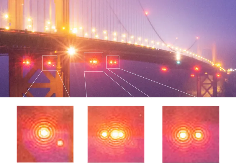
Top: Photo of the Golden Gate Bridge at night. Bottom: Zoom-in views of the red lights featuring Airy disc patterns. Captured with a Nikon D610, 27 mm lens, 30 sec exposure, f/22, ISO 400.
The photo above shows the bridge during the blue hour. The lights from the yellow sodium lamps are gently diffused by the fog. Classic star-like shapes indicate a very closed camera aperture. As for now, the photo doesn’t look very different from many others. However, if you look carefully, there’s an additional pattern coming from the red beacon lights, distinct from the spikes.
This is the Airy diffraction pattern, familiar to many physics students, though often only discussed in classes when dealing with single light sources or idealized setups. It’s fascinating to see that even in ordinary photographs, we can discover real physics at work.
What are these discs, and how do they form?
The Airy disc
Airy’s disc, a classic diffraction pattern, emerges from the interference of light. The captured light enters the camera lens and hits the sensor through the aperture, which the photographer can adjust to regulate the flow of light hitting the sensor. When the aperture is very narrow, as in this case, some of the light from the bridge diffracts before reaching the sensor. Since the aperture still has a finite size, light from different parts of the aperture follows slightly different paths before reaching the camera sensor. This causes the waves to acquire different phases and interfere, ultimately producing the characteristic pattern.
Since the aperture is almost circular, the resulting diffraction pattern is known as an Airy disk. However, the same principle applies to differently shaped apertures, leading to different diffraction patterns. A brief derivation of Airy’s disc can be found in Wikipedia.
The intensity of the Airy disk, which is what we are observing, is determined by this simple expression: $$ \begin{equation} I(r) = I_0 \left [ \frac{2J_1(x)}{x} \right ]^2, \end{equation} $$ where \( I_0 \) is the intensity of the central maximum of the pattern, \( J_1 (x)\) is the Bessel function of the first kind, \( x = ka \sin \theta \) with \(k= 2\pi/\lambda\) is the wave number and \(a\) is the aperture radius. When the angle is small, \(\sin \theta = r/d\), where \(r\) is the radius of a dark fringe and \( d \) is the distance where the light is coming from. For a light source at infinity, \(d=f\), with \(f\) the focal lenght of the lens. Thus we can relate \(x\) to the radius of the dark fringe \(r\): $$ \begin{equation} x = ka \sin \theta \simeq \frac{\pi r}{\lambda N}, \end{equation} $$ where \(N= f/2a\) is the f-number of the lens. Therefore, minima of the fringes occur when \(J_1(x\)) approaches zero, corresponding to the \(x\) zeros of the Bessel functions.
Let’s do now a little physics experiment with our photographs and explore what we can learn from them.
Load and import the diffraction pattern
For the next steps, I will work in a Python Jupyter notebook. I will also use some packages that you can find below and try to keep the code as self-explanatory as possible.
import numpy as np
import xarray as xr
import matplotlib.pyplot as plt
import proplot as pplt
from scipy.special import jn_zeros
First, we export the image in .jpg format, crop it to isolate an Airy disk and load it into the notebook.
def load_and_prepare(path, channel, x0, y0):
    """Loads an image, adjusts coordinates, and selects a channel."""
    img = xr.DataArray(plt.imread(path))
    img = img.assign_coords({'dim_0': img.dim_0.values - x0, 'dim_1': img.dim_1.values - y0})
    return img, img.sel({'dim_2': channel})

path = 'your_path_to_image'
img, img_g = load_and_prepare(path, channel=1, x0=29, y0=29)
img.plot(col='dim_2', cmap='Greys_r');
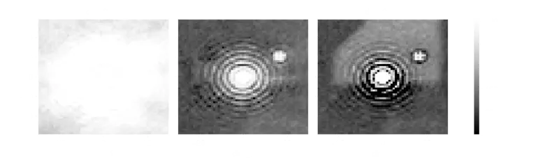
Greyscale imagse of the red, green and blue channels of the image featuring the Airy pattern.
As you can see, the img.plot() function will generate three plots. Each plot corresponds to a value in dim_2, which stores the RGB channel information in 8 bits (256 values from 0 to 255), with dim_2 = 0, 1, 2 representing R, G, B. Meanwhile, dim_0 and dim_1 store the number of pixels. The disc has been centred on the coordinate \((0,0)\). Note that the green channel contains most of the information, and we will continue to use only the data stored in img_g.
Extract the dark fringe radii
We extract the minima from the fringes (in this case manually for convenience), and store the results in the r_array dataset. Since the fringe sizes are expressed in pixels, we need to determine their actual physical dimensions on the camera sensor. My Nikon D610 has a sensor with a pixel pitch of 5.95 μm: this means that 1 pixel physically corresponds to 5.95 microns on the sensor.
Let’s now plot the single green channel with overlapping circles representing the radii of the experimentally extracted dark fringes.
pixel_size = 5.95e-6  # meters

# Experimental radii
r_array = np.array([4, 6, 9, 12, 15, 18, 20, 23]) * pixel_size
r_array = xr.DataArray(r_array, coords={'m': np.arange(1, len(r_array) + 1)})

# Plot the single green image channel
fig, ax = pplt.subplots()
ax.pcolor(img_g, cmap='Greys_r', discrete=False)

# Overlay circles with radii from the experimental data
for r in r_array.values / pixel_size:
    ax.add_patch(plt.Circle((0, 0), r, color='C2', alpha=0.7, lw=1, fill=False))
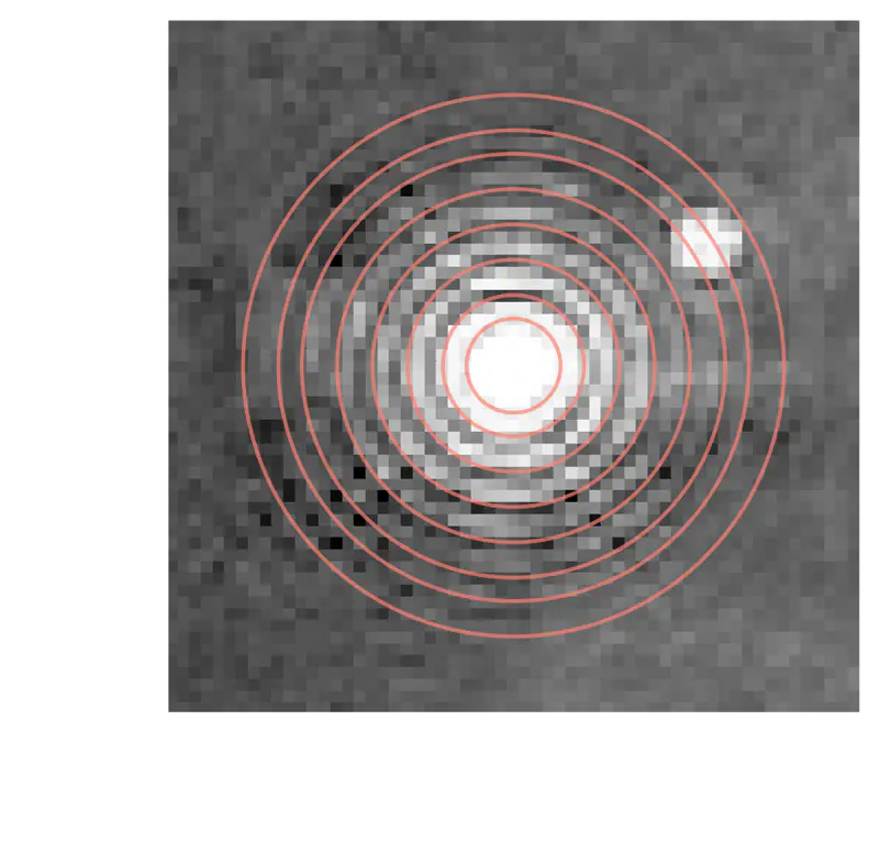
Greyscale image of the green channel of the Airy disc with overlaid eight extracted radii.
Extract the wavelength
We can now compare the experimental radii with those predicted by the equations \((1)\) and \((2)\). Each different radius \(r_n\) will correspond to a different zero \(x_n\) of the Bessel function \(J_1(x)\). We can fit the eight extracted radii to those theoretically predicted and determine the wavelength \(\lambda\) of the incoming radiation.
N = 22 # f-number

# Fit radii with predictions
def r_theory(x, wavelength, N):
    """Calculates theoretical radii based on wavelength and f-number."""
    return wavelength * N / np.pi * jn_zeros(1, len(x))

fit = r_array.curvefit('m', lambda x, wavelength: r_theory(x, wavelength, N))
lambda_theo = fit.curvefit_coefficients.values[0]

# Plot experimental data with error bars and fitted model
fig, ax = pplt.subplots()
ax.errorbar(r_array.m, r_array * 1e6, yerr=1 * pixel_size * 1e6, fmt='o', color='C3')
ax.plot(r_array.m, r_theory(r_array.m, lambda_theo, N=N) * 1e6, label=f'$\lambda$ = {lambda_theo * 1e9:.0f} nm')
ax.format(xlabel='Bessel zeros', ylabel='Radius (um)', xticks=1)
ax.legend()
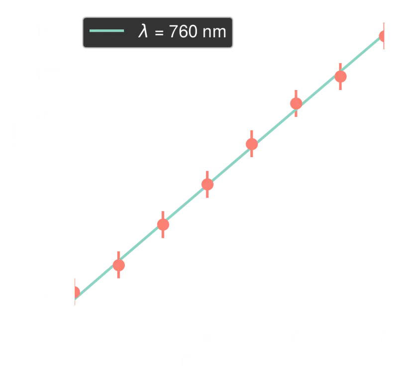
Experimentally extracted radii in red. Theoretical expectations in green are derived from the zeros of the Bessel function.
From our model, we extract \(\lambda \simeq 760~\text{nm}\), which is indeed a red light color. Congratulations! You now have a spectrometer! :-)
Conclusions
Despite the simplicity of our discussion, it is remarkable how physical phenomena can appear unexpectedly even in everyday situations and how much we can learn from them.
An even more interesting fact is that we can also work in reverse: if we know the wavelength of a known light source, we can measure the pixel size of our camera’s sensor. This is quite amazing: with a simple image, we can measure a physical length of our sensor that goes down to the scale of the micrometer!
In physics, we often find ourselves in situations where we do not know how to measure a quantity directly. However, we often know how quantities are related to each other due to some fundamental physical property and can derive them from each other.
Further thinking
If you enjoyed the discussion, I’m leaving some nice questions here for you to think about.
- Why do we need low apertures (high f-numbers) to see the interference?
- Why don’t all lights in the photos show Airy discs? What can we say about the lights used in the Golden Gate Bridge?
- How can we know if our aperture is not really circular?
- What influences the visibility of fringes? Is the light from the lamp phase coherent?
- Why is the green channel in the image the most sensitive?
- Is the distance from the object to the camera relevant in our discussion?
- I’m a photographer. Should I shoot pictures at very low apertures?